When working on data science projects, measuring a model's performance is key to determine whether the resulting model is ready to make it to production. However, one key factor that is barely taken into account when carrying out said measurements is incorporating business metrics into the model training and fine tuning process. This approach not only aligns technical outputs with business objectives but also bridges the gap between data science teams and business stakeholders. It also ensures that machine learning initiatives are not just technically sound but also strategically significant, fostering a data-driven culture where insights are actionable and investments in AI and machine learning yield substantial returns.

This strategy is applicable in different fields, such as predicting the severity of an illness to correctly allocate medical resources for treatment or predicting demand on perishable goods to minimize waste and maximize gains. To demonstrate how we can make use of these business defined metrics we will be training a model on the Credit Card Fraud Detection dataset which contains real, yet anonymized, credit card transactions. This is a typical binary classification problem with a highly imbalanced dataset, where our main goal is to predict if a transaction is fraudulent or not.

In a usual machine learning workflow we would start by defining the target metrics to optimize when training the model. Given the type of problem, we would use metrics like the F1 score, precision, recall or Matthew’s correlation coefficient. However, more often than not, when sharing results with stakeholders most data scientists simply rely on indicating that if there is an uplift in X metric, that means we have a better model. But stakeholders speak KPIs and business metrics. For this problem, we will measure a model’s performance in terms of Net Gain, being defined as:

Net Gain =Transaction Amount * Fee Percentage- Fraudulent Transaction Amounts

Assuming we are a credit card provider, we would charge a fixed rate on each transaction, let’s say 2%. On the other hand, for each fraudulent transaction its entire amount represents a loss to our business. We now need to determine how we plug it in our model training process. In order to do so, we first need to reason how our model would impact the business when in production:

• If our model predicts the transaction as non fraud and:
  • It isn’t fraudulent (a true negative): we’d earn that transaction’s fee
  • It is fraudulent (a false negative): we’d earn that transaction’s fee, but lose the entire transaction’s amount
• If our model predicts the transaction as fraud and:
  • It is fraudulent (a true positive): we’d lose that transaction’s fee (but we would have avoided the loss of the entire transaction’s amount)
  • It isn’t fraudulent (a false positive): we’d lose that transaction’s fee

By following the aforementioned rules, we can compute the Net Gain at a transaction level. We then sum up each transaction’s Net Gain to get the overall metric value. This is a special case of cost-sensitive learning.

Time to implement this in code. Let’s start with the setup, a basic requirements.txt file:

pandas==2.2.2
scikit-learn==1.4.2
xgboost==2.0.3

For the sake of simplicity, we will skip all the exploratory data analysis and jump directly into training the model. First, let’s import all the required libs:

from typing import Iterable

import numpy as np
import pandas as pd
from numpy.typing import NDArray
from sklearn.model_selection import StratifiedKFold
from xgboost import XGBClassifier

Now, we’ll load the data and split it into the training and testing sets:

data = pd.read_csv("creditcard.csv")

splitter = StratifiedKFold(shuffle=True, random_state=42)
train_ix, test_ix = next(splitter.split(data, data["Class"]))

train = data.iloc[train_ix]
test = data.iloc[test_ix]

X_train = train.drop(columns=["Time", "Class"])
X_test = test.drop(columns=["Time", "Class"])
y_train = train["Class"].values

# We'll also keep the amount in the testing
# ground truth so we can compute the net gain
# later
y_test = test[["Amount", "Class"]].values

Next, let’s establish the baseline, which is the Net Gain of the business without the model:

FEE_RATE = .02

total_loss = test[test["Class"] == 1]["Amount"].sum()
total_earnings = test["Amount"].sum() * FEE_RATE
net_gain = total_earnings - total_loss

print(f"Total earnings: {total_earnings:>12.2f}")
print(f"Total fraud losses: {total_loss:.2f}")
print(f"Net gain: {net_gain:>18.2f}")

>>> Total earnings:      98730.76
>>> Total fraud losses: 15186.50
>>> Net gain:               83544.26

Our goal will then be to produce a Net Gain higher than $83,544.26 using our model. But before training the model, we need to define our function to compute the business metric:

def compute_net_gain(
    y_true: NDArray[tuple[float, int]],
    y_preds: NDArray[int],
) -> float:
    net_gain = 0
    for (amount, class_), y_pred in zip(y_true, y_preds):
        # True positive
        if y_pred == class_ == 1:
            net_gain -= amount * FEE_RATE

        # True negative
        elif y_pred == class_ == 0:
            net_gain += amount * FEE_RATE

        # False positive
        elif y_pred != class_ == 0:
            net_gain -= amount * FEE_RATE

        # False negative
        elif y_pred != class_ == 1:
            net_gain += amount * FEE_RATE - amount

    return net_gain

With that in place, let’s train an eXtreme Gradient Boosting algorithm on our training dataset, generate predictions for our testing dataset and finally plug the generated predictions as well as the testing ground truth into our previously defined function:

clf = XGBClassifier(random_state=42).fit(X_train, y_train)
y_pred = clf.predict(X_test)
compute_net_gain(y_test, y_pred)

>>> 94543.086

Should our model have been in production, the company’s Net Gain would have been $94,543.086, an outstanding 13.16% lift from the $83,544.26 baseline.

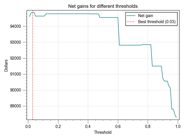
Finally, we can do a threshold adjustment to maximize the gains and pick the best cutoff value:

y_probs = clf.predict_proba(X_test)[:, 1]
net_gains = []

thresholds = np.arange(.01, 1, .01)
for threshold in thresholds:
    y_pred = (y_probs >= threshold).astype(int)
    net_gain = compute_net_gain(y_test, y_pred)
    net_gains.append(net_gain)

max_gain = max(net_gains)
best_threshold = thresholds[net_gains.index(max_gain)]
print(f"Max net gain: {max_gain:.3f}\nat threshold: {best_threshold}")

>>> Max net gain: 94865.504
>>> at threshold: 0.03

By using a .03 threshold, we now achieve a Net Gain of $94,865.50, representing a 13.55% lift from our baseline.

Communicating the 13.55% net gains lift is more impactful than detailing machine learning metrics like F1 or precision. This tangible financial improvement directly resonates with stakeholders, clearly demonstrating the model's value in enhancing profitability and operational effectiveness. This approach aligns with business goals, making the benefits of our data science solutions easily understandable and relevant to decision-makers.